SingleMeasure

read.csv(file = "../data-raw/IUCN Red List Changes - 2002 to 2022 - Single Measure.csv") -> Single_Measure
read.csv(file = "../data-raw/IUCN Red List Changes - 2002 to 2022 - Multiple Measures.csv") -> Multiple_Measure

head(Single_Measure)

##   Year      Class                Metric Number.of.Species
## 1 2002 Amphibians Critically Endangered                30
## 2 2003 Amphibians Critically Endangered                30
## 3 2004 Amphibians Critically Endangered               413
## 4 2006 Amphibians Critically Endangered               442
## 5 2007 Amphibians Critically Endangered               441
## 6 2008 Amphibians Critically Endangered               475

Single_Measure %>% 
  filter(Class == "Amphibians" | Class == " 
Birds" | Class == "Fishes" | Class == "Fungi & Protists") %>% 
  group_by(Class, Metric) %>% 
  head()

## # A tibble: 6 × 4
## # Groups:   Class, Metric [1]
##    Year Class      Metric                Number.of.Species
##   <int> <chr>      <chr>                 <chr>            
## 1  2002 Amphibians Critically Endangered 30               
## 2  2003 Amphibians Critically Endangered 30               
## 3  2004 Amphibians Critically Endangered 413              
## 4  2006 Amphibians Critically Endangered 442              
## 5  2007 Amphibians Critically Endangered 441              
## 6  2008 Amphibians Critically Endangered 475

Taking a look at species that are in danger of becoming endangered

#as.integer(Single_Measure$Number.of.Species)
Single_Measure %>% 
  group_by(Metric) %>%
  mutate(Species = as.integer(Number.of.Species)) %>% 
  filter(!is.na(Species)) %>% 
ggplot(mapping = aes(x = Year, y = Species, color = Metric)) +
  geom_point(size = 0.5) +
  facet_wrap(~Class, scales = "free_y")

## Warning: There was 1 warning in `mutate()`.
## ℹ In argument: `Species = as.integer(Number.of.Species)`.
## ℹ In group 3: `Metric = "Total Assessed"`.
## Caused by warning:
## ! NAs introduced by coercion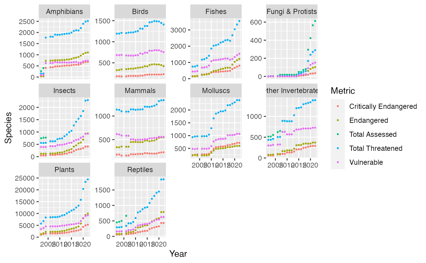

str(Single_Measure)

## 'data.frame':    1000 obs. of  4 variables:
##  $ Year             : int  2002 2003 2004 2006 2007 2008 2009 2010 2011 2012 ...
##  $ Class            : chr  "Amphibians" "Amphibians" "Amphibians" "Amphibians" ...
##  $ Metric           : chr  "Critically Endangered" "Critically Endangered" "Critically Endangered" "Critically Endangered" ...
##  $ Number.of.Species: chr  "30" "30" "413" "442" ...

Trends that show the rate of extinct for each species. Amphibians, Birds, fishes, insects, Mammals, Molluscs, Invertebrate, Plants, reptiles have graphs that show that these species are threatened to go instinct. While Fungi and protist is the largest group that has been assessed

Single_Measure %>% 
  filter(Class == "amphibians" | Class == "Mammals" | Class == "Fungi & Protists" | Class == "Mollus" | Class == "Reptiles" | Class == "Plants" | Class == "Other Invertebrates") %>% 
  group_by(Metric) %>% 
  mutate(Species = as.integer(Number.of.Species)) %>% 
  filter(!is.na(Species)) %>% 
  ggplot(mapping = aes(x = Year, y = Species, color = Metric)) +
  geom_point(size = 1) +
  facet_wrap(~Class, scales = "free_y")

## Warning: There was 1 warning in `mutate()`.
## ℹ In argument: `Species = as.integer(Number.of.Species)`.
## ℹ In group 3: `Metric = "Total Assessed"`.
## Caused by warning:
## ! NAs introduced by coercion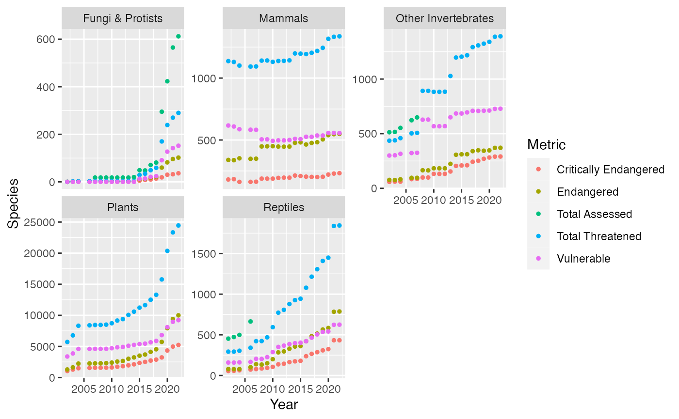

Single_Measure %>% 
  mutate(Species = as.integer(Number.of.Species)) %>% 
  group_by(Year, Class) %>%
  filter(!is.na(Species)) %>% 
  filter(Class == "Birds") %>% 
  summarize(bird_mean = mean(Species))

## Warning: There was 1 warning in `mutate()`.
## ℹ In argument: `Species = as.integer(Number.of.Species)`.
## Caused by warning:
## ! NAs introduced by coercion

## `summarise()` has grouped output by 'Year'. You can override using the
## `.groups` argument.

## # A tibble: 20 × 3
## # Groups:   Year [20]
##     Year Class bird_mean
##    <int> <chr>     <dbl>
##  1  2002 Birds      596 
##  2  2003 Birds      597 
##  3  2004 Birds      606 
##  4  2006 Birds      603 
##  5  2007 Birds      608.
##  6  2008 Birds      611 
##  7  2009 Birds      612.
##  8  2010 Birds      620 
##  9  2011 Birds      626.
## 10  2012 Birds      656.
## 11  2013 Birds      654 
## 12  2014 Birds      686.
## 13  2015 Birds      688.
## 14  2016 Birds      730 
## 15  2017 Birds      734.
## 16  2018 Birds      746 
## 17  2019 Birds      743 
## 18  2020 Birds      740.
## 19  2021 Birds      722.
## 20  2022 Birds      704.

Taking look at birds which are closely related to reptiles and seeing how the average of birds have changed throughout the years